16 Ops for the extraction
16.1 First time: preparing a PC
16.1.1 Installing the software
Whether you need to install any software for the extraction is mostly a matter of personal preference. You will need to validate every extraction script to make sure you didn’t accidently make a typo (e.g. forgot a quote) or extracted an entity in the wrong format.
One option is to do this using EVA (the Extraction Validation App), at https://opens.science/apps/eva. In that case, the only software you need is an application to edit plain text files. You can use whatever came with your operating system (e.g. Notepad in Windows, Text Edit in MacOS, or GNOME Text Editor in Ubuntu). You can also install a more powerful text editor, like Notepad++.
Alternatively, you can use RStudio and R. This has two advantages over the approach discussed in the last paragraph. First, you have the benefit of RStudio’s syntax coloring. This is very helpful to help you avoid accidentily omitting a quote or a parenthesis. In addition, you can then directly validate your extraction by ‘knitting’ or ‘rendering’ the R Extraction Script in R. If you want to use R and RStudio, you have to install these programs if they are not present yet:
For all three programs, you can accept the default options in the installation, but for Git, you may want to select that you use Notepad (or Notepad++ if you have it) as the default editor instead of Vim; and you may want to select “main” as default branch name instead of “master”.
16.1.2 Installing the R packages
If you want to use R, you will also need to install a number of R packages. Once you installed R and RStudio, start RStudio and then run these commands by copying them and pasting them in the console (the bottom-left panel in RStudio):
install.packages(c('remotes', 'here', 'markdown', 'commonmark'),
                 repos='http://cran.rstudio.com');
install.packages(c('ufs', 'ggplot2', 'DiagrammeR', 'DiagrammeRsvg'),
                 repos='http://cran.rstudio.com');
install.packages(c('yum', 'synthesisr', 'preregr', 'rock'),
                 repos='http://cran.rstudio.com');
ufs::quietGitLabUpdate("r-packages/metabefor", quiet = FALSE);
The last of these installs the {metabefor} package from its Git repository. Once {metabefor} is on CRAN, you can install from there using install.packages().
16.1.3 Cloning the repository
Cloning means that you copy a Git repository to your local PC. This will download all files in the project, along with the metadata needed to pull from and push to the server (e.g., a GitLab or Codeberg server).
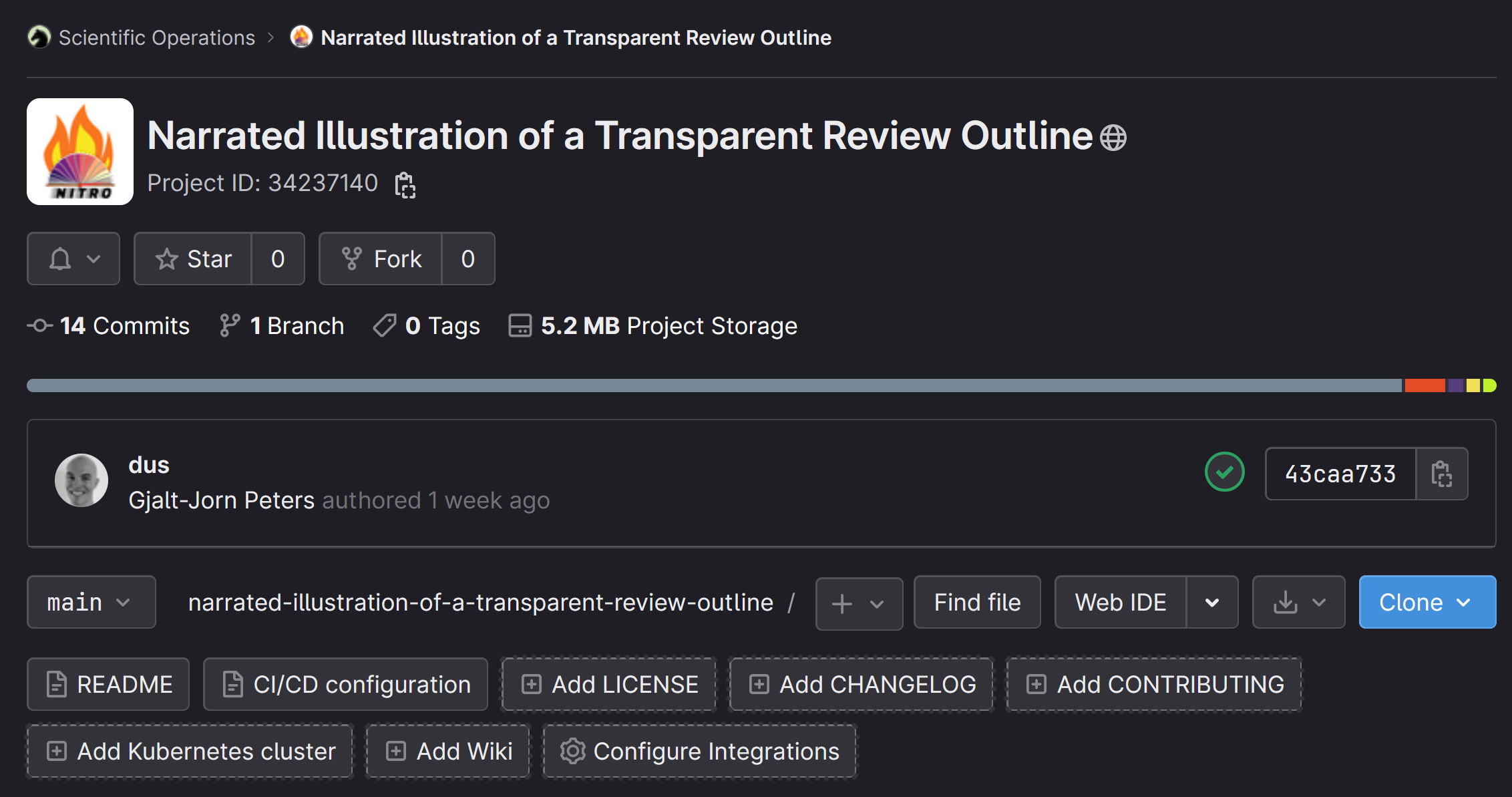
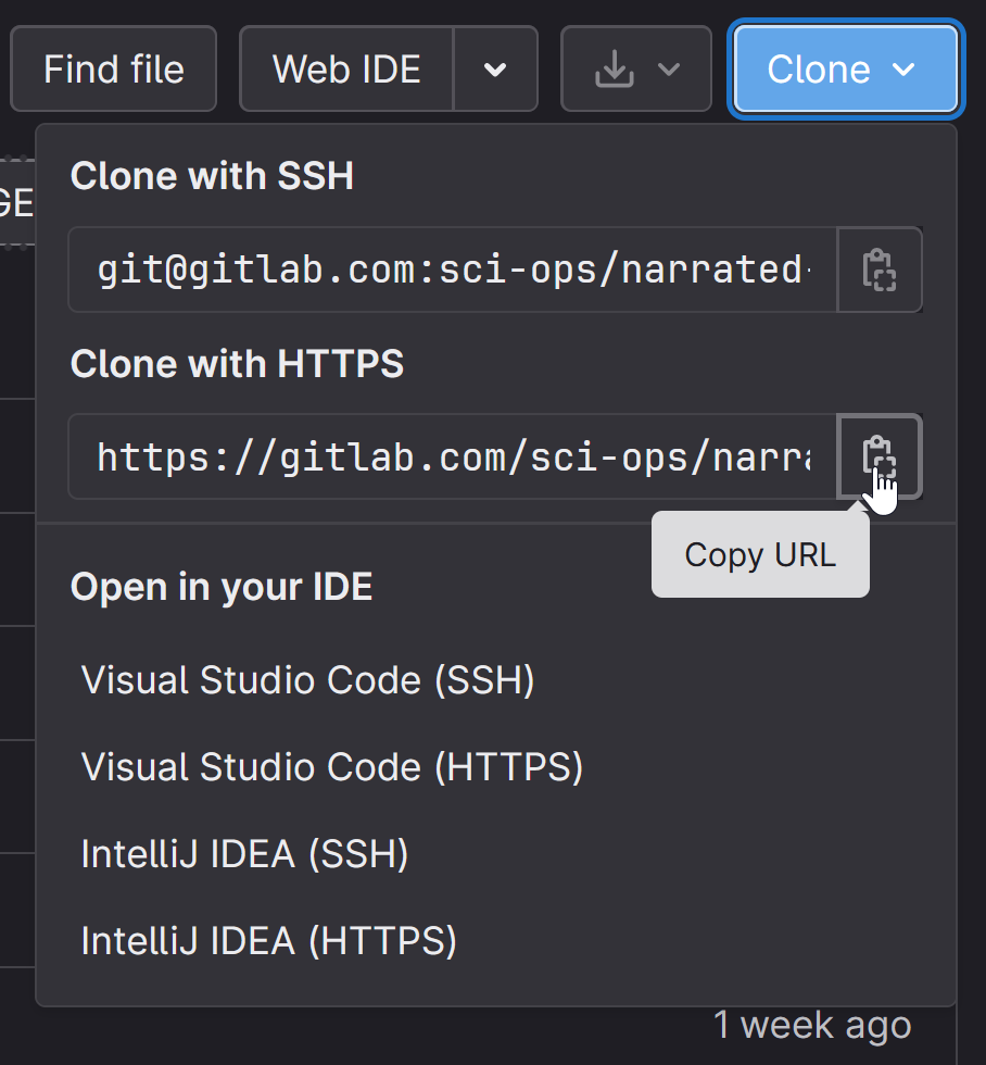
In your browser, navigate to the URL of the Git repository (e.g., the URL of the NITRO repository). There, click the “Clone” button.
In RStudio, klik links bovenin op “File” en dan “New Project”
Kies “Version Control” en dan “Git”
Copy-paste de URL
Druk op Tab; hiermee gaat de cursor naar het volgende veld waar de directorynaam wordt gespecificeerd. Als het goed is “autovult” hij die met de naam van het repository (in bovenstaand voorbeeld, “verlicht-scoping-review-1”)
Kies in het derde veld een plaats om die directory aan te maken en het project naartoe te ‘clonen’. Neem bij voorkeur een lokale directory, dus niet een subdirectory van een directory van een cloud-dienst (e.g. OneDrive, DropBox, etc). Bij de OU zijn de Documenten directory en de Desktop wel subdirectories van een synchronisatiedienst (met de OU server), dus als je op een OU laptop zit, kies dan een directory op de D-drive. R opent nu je project.
16.2 For every source
- Open the source you want to extract (e.g. a PDF of an article)
- Look up the unique source identifier for this source. If the source has a DOI, then go to https://shortdoi.org to produce the corresponding ShortDOI. If it doesn’t have a DOI, the source identifier is the QURID, which you can get from the bibliographic database you used for the screening.
- Open RStudio or whichever text editor you use
- Navigate to the directory holding the Rxs template (probably “
extraction-Rxs-spec”) - Open this file.
- Save it again with a new name, specifically a name constructed as follows:
- Family name first author (with all characters other than Latin leters (a-z) removed)
- An underscore (
_) - sourceId (shortdoi or QURID)
- An underscore (
_) - Year of publication of the source
- An underscore (
_) - Extractor identifier (your identifier)
- The extension (
.rxs.Rmd)
- An example filename is
batty_2020_j58m_fm2.rxs.Rmd - Then, start completing the Rxs file: scroll through it from top to bottom, and insert the value of every entity that you extract from the PDF
- If you use Git, then once you’re done, you can push your Rxs file with:
git pull; git add . ; git commit -m "Commit boodschap" ; git push
16.3 Coding an extracted entity
When planning the extraction, you decided for each entity where on the coding-categorization continuum you would extract it (see Chapter 6). The entities that you decided to extract literally from the sources have to be coded.
This coding consists of attaching code identifiers to the entity values for a given entity. If you code entities, the extracted values will almost always be literal text strings that were integrally copied from the sources.
Examples of entities that you may choose to extract integrally and then code are the definitions authors use for a concept; or their description of their sampling procedure; or their reasoning underlying a certain decision; or the way they phrase the research questions or their conclusions.
During the coding, you look for patterns in these extracted texts, and you then attach codes to make those patterns machine-readable (which will make it possible to combine this information with the other information you extracted).
16.3.1 Your codebook
As you attach more codes, you develop your codebook. A codebook is a document that defines each code. Typically, for each code, you document the following:
- A code identifier: Like entity identifiers, these can only consist of lower and upper case Latin letters (
a-zandA-Z), Arabic digits (0-9), and underscores (_), and must always start with a letter. Valid identifiers aresocialNorms,broadConclusion,conditionalStatement,sampling_purposive, andrhetoric_authorityArgument. - A code label: This is a very short human-readable title for the code. Unlike identifiers, labels are pretty much unconstrained, so valid labels are
Social Norms,Drawing of a Broad Conclusion,Statement conditional upon other statement,Sampling strategy: purposive, andRhetoric: use of authority argument. - A code description: This is a longer description of the concept captures by the code. This can be quite long, multiple paragraphs even, and will typically become more comprehensive as you code more data and so develop your codes further and further. The code description determines when a code applies to a given bit of data, together with the coding instruction.
- A coding instruction: This is an explicit instruction as to when this code should be attached to a data fragment. Unlike the code description, which describes the concept that the code captures (e.g. a psychological construct, or a procedural element of a study, or a reasoning strategy), the instruction is very operational. It described what a coder should look for in the data to decide whether this code should be applied. It typically also describes edge cases and uses those to refer to other codes, for example: “Use this code for expressions that relate directly to authors’ expectations regarding the outcome variables of the study. However, do not use this code for expectations regarding variables that are included in the design as predictors or covariates. In those cases, instead attach the codes with identifiers
expect_varPredictorandexpect_varCovariate.”
In addition to these four basic characteristics, it is often beneficial to include examples of data that should or should not be coded with the code. Specifically, it is helpful to include four types of examples:
- examples of data fragments that should be coded with the code according to the code description and coding instructions (matches);
- examples of data fragments that should not be coded with the code according to the code description and coding instructions (mismatches);
- examples of data fragments that are relatively ambiguous to classify (edge cases);
- examples of data fragments that are very easy to classify (core cases);
Developing these four types (core case matches, core case mismatches, edge case matches, and edge case mismatches) help establish what you consider to be clear core examples of what should and should not be coded, as well as where the codes’ conceptual boundaries lie.
An example of a codebook in spreadsheet format is available here. Note that this example is for a codebook as applied to qualitative data as produced in individual interviews with participants, so the types of codes will probably be quite different from the types of codes you use in systematic reviews.
When developing your codebook, you aim to describe the codes so explicitly, accurately, and comprehensively that others can also use the codebook. Ideally, everybody who uses the codebook codes the data in the same way. If there are resources for this in your project, it pays to have multiple coders and develop the codebook together. If you manage to create a codebook that indeed can be applied by others to arrive at the same codings (i.e. the same codes applied to the same data fragments), you know you have described the codes sufficiently clearly to be transparent about the relevant parts of the data as captures by the codes.
16.3.2 Inductive versus deductive coding
Coding occurs on a spectrum from fully inductive to fully deductive, with most cases being somewhere in the middle.
Fully inductive coding means you have no preliminary ideas about what kind of codes you may encounter. This is also called ‘open coding’. In this case you start without a codebook, and you create the codebook as you develop your codes from scratch.
Fully deductive coding means you start out with a full codebook. If you really only code deductively, that implies that the codebook will not be updated, because such updates suggest that you still learn about the concepts you’re coding, which would suggest you work partly inductively after all. In the context of a systematic review, it’s unlikely (but not impossible) that you decide to code an entity deductively. After all, if you already know pretty much everything about it, you can often capture this knowledge in categorical entities, and so you categorize upon entity extraction (and do not extract raw source data such as text strings).
Often, you have some idea as to which codes you’ll probably use, but you’re also often open to changing these (maybe even completely if necessary), so it’s quite common to have a very rudimentary codebook when you start coding, but to heavily develop this further during coding.
16.3.3 Coding in the ROCK standard
The {metabefor} package can export entities to and from the ROCK format (see this manual page). The ROCK format is the format for the Reproducible Open Coding Kit: a standard to store coded qualitative data in a format that is simultaneously human- and machine-readable (for more information, see http://rock.science).
When importing ROCK data that was previously exported by the {metabefor}, the codes can be combined with the other extracted data. This realizes a fully transparent process, where it is clear which raw data were coded, which codes were applied to which entities (using which codebook), and how these are combined with the rest of the extracted data.
The ROCK standard consists of plain-text files (just like .Rxs.Rmd files are plain text files). These can be opened with any software that can edit text files, such as RStudio, Notepad++, or stock applications that come with your operating system, such as Notepad on Windows and TextEdit on MacOS. To code a data fragment with a code, simply add the code identifier for that code at the end of the same line as the data fragment, in between two square brackets.
This is an example of a coded data fragment:
This is some text in the fragment. [[this_is_a_code_identifier]]It is also possible to attach multiple codes:
This is some other text fragment. [[code1]] [[code2]]This is an example of some exported and then coded entity values:
[[rxsSourceId=gpg36g]]
[[rxsEntityId=population]]

hotel employees on the Canary Islands [[employees]]


[[rxsSourceId=qurid_7pdb7n68]]
[[rxsEntityId=population]]

undergraduates from a public university [[students]]


[[rxsSourceId=gnt2hz]]
[[rxsEntityId=population]]

healthcare professionals working in a in a hospital in the Northern Italy [[employees]]


[[rxsSourceId=knfh]]
[[rxsEntityId=population]]

employees of an Italian subsidiary of a European multinational company  [[employees]]
        active in the food producer sector
The two codes at the start of every fragment are added by the {metabefor} package when it exports the entity values to the .rock file. The rxsSourceId is the source identifier of the source from which the following entity value was extracted. The rxsEntityId is the identifier of the entity from that that entity value was extracted (in this case, we’re coding the authors’ description of the population they studied).
The codes that were added by the researcher have code identifiers students and employees, and the fact that these are not just words (parts of the data) but codes that have been attached to the data is signified by the double square brackets surrounding each code identifier.
During coding, the things that costs most time is thinking. Thinking about whether a given code applies; thinking about whether the code book should be updated; and if so, how. The time you spend actually attaching the code is often negligible compared to the time you need for thinking. Coding is mostly an intellectual effort, and the operational side (i.e. adding the code identifier to the .rock file) is relatively small. Therefore, often you might as well type the code identifier in a text editor. However, if you want, there is a rudimentary interface to add codes called iROCK. You can access it at https://i.rock.science. If you use iROCK, make sure you download the coded file again and store it locally: if you forget to download it and close your browser, you lose all your work. A part of the workshop about the ROCK explains how to work with iROCK, in case you want more information: https://rock.science/workshop/2hr.
16.3.4 After the coding
Once you finished coding a source, it can be imported again and the codes will be added to the rest of the extracted data. You can then include this in datasets you want to extract from the object with extracted data. If you are doing this as a student, your supervisor will most likely handle the importing and the production of the dataset, which they will then send to you in .xlsx, .csv, .obv, or .sav format.